Survival Model Evaluation Methods

stats_misc.machine_learning.sksurv_utils provides helpers for extracting predictions, evaluating discrimination, and assessing calibration from scikit-survival models. We will also show how the module functions can be generalised to take scikit-survival compliant input data, forgoing the need for sksurv model objects.

import matplotlib.pyplot as plt
import numpy as np
import pandas as pd
from matplotlib.lines import Line2D
from sklearn.model_selection import train_test_split
from sksurv.datasets import load_whas500
from sksurv.linear_model import CoxPHSurvivalAnalysis
from sksurv.nonparametric import kaplan_meier_estimator, nelson_aalen_estimator
from sksurv.util import Surv

from stats_misc.machine_learning.sksurv_utils import (
    SurvivalModelBrierScore,
    SurvivalModelCalibration,
    event_by_time,
    surv_model_auc,
    surv_model_calibration_table,
    surv_model_predict,
)

Data and model

We use the Worcester Heart Attack Study dataset (WHAS500, 500 patients) shipped with scikit-survival. The outcome is all-cause mortality with follow-up recorded in days.

The structured outcome array is renamed to the standard event/time field convention expected by sksurv_utils functions.

X_df, y_raw = load_whas500()

# Convert to numpy and rename outcome fields to the 'event'/'time' convention.
X = X_df.to_numpy()
y = Surv.from_arrays(y_raw['fstat'].astype(bool), y_raw['lenfol'])

print(f'Patients: {X.shape[0]}\nFeatures: {X.shape[1]}')
print(f'Event rate: {y["event"].mean():.2%}')
print(f'Follow-up range: {y["time"].min():.0f}\u2013{y["time"].max():.0f} days')

Patients: 500
Features: 14
Event rate: 43.00%
Follow-up range: 1–2358 days

X_train, X_test, y_train, y_test = train_test_split(
    X, y, test_size=0.2, random_state=42
)
print(f'Train: {X_train.shape[0]}, Test: {X_test.shape[0]}')

model = CoxPHSurvivalAnalysis()
model.fit(X_train, y_train)
print('Cox proportional hazards model fitted.')

# Evaluate at 1, 2, 3, and 4 years post-admission.
times = [365.0, 730.0, 1095.0, 1460.0]

Train: 400, Test: 100
Cox proportional hazards model fitted.

Risk predictions at fixed time points using surv_model_predict

Returns a DataFrame with one column per time point containing predicted event risk (1 − survival probability) for each subject.

risk_df = surv_model_predict(model, X_test, times)
risk_df.head()

	Predicted risk at 365.0	Predicted risk at 730.0	Predicted risk at 1095.0	Predicted risk at 1460.0
0	0.077677	0.118249	0.135798	0.174164
1	0.341441	0.478001	0.529490	0.627872
2	0.057534	0.088098	0.101434	0.130845
3	0.081812	0.124394	0.142779	0.182900
4	0.529695	0.690894	0.743755	0.832249

Time-dependent discrimination using surv_model_auc

Computes cumulative/dynamic AUC at each time point using cumulative_dynamic_auc from scikit-survival.

The data argument is a tuple of (label, test_y, test_x_or_predictions). When model is provided, the function calls model.predict() internally; when model=None, the third element is used directly as pre-computed risk scores.

train_y is required to estimate the censoring distribution. The cumulative/dynamic AUC handles right-censored observations using inverse probability of censoring weights (IPCW), where the weights are derived from a Kaplan–Meier estimate of the censoring distribution. Ideally these weights are estimated from the training data (which often is larger than the X% testing data).

In external validation setting the original training data might not be available. In such setting one could consider simply parsing the same y_test object to the train_y parameter. This will not introcude any kind of overfitting or model optimism, the underlying Kaplan-Meier is fully non-parametric, but it does introduce covariance between the IPCW weights and the event indicator, affecting the efficiency of the variance estimator. Dependingon the number of available observations this lack of efficiency may be trivial.

auc_results = surv_model_auc(
    model=model,
    times=times,
    data=('test', y_test, X_test),
    train_y=y_train,
)
print(auc_results)

       Data split  AUC by time  Mean AUC
Time
365.0        test     0.739679  0.754461
730.0        test     0.771122  0.754461
1095.0       test     0.792971  0.754461
1460.0       test     0.714072  0.754461

User-supplied predictions

When model=None, the caller supplies pre-computed risk scores directly. This is useful when predictions come from a pre-existing prediction rule and may not be based on an sksurv model. As mentioned above, in such a setting one typically does not have access to the training Y array and we therefore use the testing array instead.

precomputed_risk = model.predict(X_test)

auc_precomputed = surv_model_auc(
    model=None,
    times=times,
    data=('test (pre-computed)', y_test, precomputed_risk),
    train_y=y_test,
)
print(auc_precomputed)

                 Data split  AUC by time  Mean AUC
Time
365.0   test (pre-computed)     0.739679  0.756472
730.0   test (pre-computed)     0.771268  0.756472
1095.0  test (pre-computed)     0.793401  0.756472
1460.0  test (pre-computed)     0.721540  0.756472

Determine whether a subject had an event for each supplied time point using event_by_time

Returns a DataFrame indicating whether each subject experienced the event by each of the specified time points.

events_df = event_by_time(y_test, times)
print(f'Cumulative event rate by time point:')
print(events_df.mean().to_string())

Cumulative event rate by time point:
Event at 365.0     0.29
Event at 730.0     0.35
Event at 1095.0    0.36
Event at 1460.0    0.37

Compare predicted risk to observed events using surv_model_calibration_table

Concatenates predicted risks (from surv_model_predict) with observed binary outcomes (from event_by_time) into a single table, one row per subject.

cal_table = surv_model_calibration_table(model, X_test, y_test, times)
print(f'Shape: {cal_table.shape}')
cal_table.head()

Shape: (100, 8)

	Predicted risk at 365.0	Predicted risk at 730.0	Predicted risk at 1095.0	Predicted risk at 1460.0	Event at 365.0	Event at 730.0	Event at 1095.0	Event at 1460.0
0	0.077677	0.118249	0.135798	0.174164	0	0	0	0
1	0.341441	0.478001	0.529490	0.627872	0	0	0	0
2	0.057534	0.088098	0.101434	0.130845	0	0	0	0
3	0.081812	0.124394	0.142779	0.182900	0	0	0	0
4	0.529695	0.690894	0.743755	0.832249	1	1	1	1

Calculate the integrated Brier score using SurvivalModelBrierScore

Evaluates a survival model using the integrated Brier score (IBS) and computes the baseline non-informative Brier score π(1 − π), enabling a Brier skill score (BSS) that measures improvement over the naive baseline.

brier_scorer = SurvivalModelBrierScore(model, np.array(times))
ibs = brier_scorer(y_train, y_test, X_test)
bss = brier_scorer.get_brier_skill_score()

print(brier_scorer)

SurvivalModelBrierScore for model: CoxPHSurvivalAnalysis
  Time points: 4 evaluated
  Integrated Brier Score (IBS): 0.1865
  Baseline Brier Score (π(1 - π)): 0.2451
  The Brier Skill Score: 0.2391

Calculate stratified calibration curves using SurvivalModelCalibration

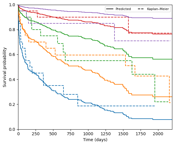
Divides subjects into risk groups based on mean predicted survival, then compares the group-average predicted survival curve against the non-parametric (Kaplan–Meier) estimate for each group.

calibration = SurvivalModelCalibration(model, n_groups=5)
durations_test = y_test['time']
events_test = y_test['event'].astype(int)

group_summary = calibration(X_test, durations_test, events_test)
print(calibration)

# Making a graph to compare predicted versus observed survival probabilities
fig, ax = plt.subplots(figsize=(6, 5))
colors = plt.cm.tab10(np.arange(len(group_summary)))

for color, (group_id, g) in zip(colors, group_summary.items()):
    ax.step(g['predicted_times'], g['predicted_survival'],
            where='post', color=color, lw=1.5)
    ax.step(g['observed_times'], g['observed_survival'],
            where='post', color=color, lw=1.5, linestyle='--')

style_handles = [
    Line2D([0], [0], color='k', lw=1.5, label='Predicted'),
    Line2D([0], [0], color='k', lw=1.5, linestyle='--', label='Kaplan–Meier'),
]
group_handles, _ = ax.get_legend_handles_labels()
ax.legend(handles=group_handles + style_handles, fontsize=8, ncol=2)
ax.set_xlabel('Time (days)')
ax.set_ylabel('Survival probability')
ax.set_ylim(0, 1)
ax.set_xlim(0, 2200)
plt.tight_layout()
plt.show()

SurvivalModelCalibration with model: CoxPHSurvivalAnalysis
  Number of groups: 5
  Estimator: kaplan_meier_estimator
  Group summary available for 5 group(s).

Nelson–Aalen (Breslow) estimator

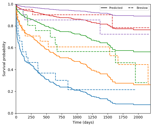
SurvivalModelCalibration accepts any callable with the signature (event, time) -> (times, survival) as its nonparametric_estimator. The Nelson–Aalen cumulative hazard estimate H(t) can be converted to a survival curve via S(t) = exp(−H(t)), which is the Breslow estimator. It is less conservative than Kaplan–Meier in small groups and may yield slightly smoother calibration curves.

def breslow_survival(event, time):
    t, cum_hazard = nelson_aalen_estimator(event, time)
    return t, np.exp(-cum_hazard)

cal_na = SurvivalModelCalibration(
    model, n_groups=5, nonparametric_estimator=breslow_survival
)
group_summary_na = cal_na(X_test, durations_test, events_test)

# making the same graph
fig, ax = plt.subplots(figsize=(6, 5))
colors = plt.cm.tab10(np.arange(len(group_summary_na)))

for color, (group_id, g) in zip(colors, group_summary_na.items()):
    ax.step(g['predicted_times'], g['predicted_survival'],
            where='post', color=color, lw=1.5)
    ax.step(g['observed_times'], g['observed_survival'],
            where='post', color=color, lw=1.5, linestyle='--')

style_handles = [
    Line2D([0], [0], color='k', lw=1.5, label='Predicted'),
    Line2D([0], [0], color='k', lw=1.5, linestyle='--', label='Breslow'),
]
group_handles, _ = ax.get_legend_handles_labels()
ax.legend(handles=group_handles + style_handles, fontsize=8, ncol=2)
ax.set_xlabel('Time (days)')
ax.set_ylabel('Survival probability')
ax.set_ylim(0, 1)
ax.set_xlim(0, 2200)
plt.tight_layout()
plt.show()

Raw survival function output

SurvivalModelBrierScore and SurvivalModelCalibration both call model.predict_survival_function(X) internally. It returns an array of StepFunction objects — one per subject — each with .x (the unique event times seen during training) and .y (estimated survival probability at those times). The array structure, subjects × time points, is the natural representation for any generalisation that bypasses the model object entirely.

surv_funcs = model.predict_survival_function(X_test)

print(f'Type:              {type(surv_funcs)}')
print(f'Length:            {len(surv_funcs)}  (one StepFunction per subject)')
print(f'Time points:       {len(surv_funcs[0].x)}  (unique event times from training)')
print(f'First 5 times:     {surv_funcs[0].x[:5]}')
print(f'First 5 S(t):      {np.round(surv_funcs[0].y[:5], 4)}')

# As a subjects × times matrix — the format needed for a model-free generalisation.
surv_matrix = np.row_stack([fn.y for fn in surv_funcs])
print(f'\nMatrix shape (subjects × times): {surv_matrix.shape}')

Type:              <class 'numpy.ndarray'>
Length:            100  (one StepFunction per subject)
Time points:       324  (unique event times from training)
First 5 times:     [1. 2. 3. 4. 6.]
First 5 S(t):      [0.9967 0.9933 0.9918 0.9908 0.9881]

Matrix shape (subjects × times): (100, 324)

/tmp/ipykernel_14320/296467557.py:10: DeprecationWarning: `row_stack` alias is deprecated. Use `np.vstack` directly.
  surv_matrix = np.row_stack([fn.y for fn in surv_funcs])